The integrate and fire neuron
In this notebook we will use Python to simulate the integrate and fire (I&F) neuron model. We’ll investigate, in particular, how the spiking activity varies as we adjust the input current \(I\).
Background information about the I&F model
Here’s a video that describes a slightly more complicated model, the leaky integrate and fire model.
from IPython.lib.display import VimeoVideo
VimeoVideo('140084447')
Here’s some additional intereting videos and references:
Preliminaries
Before beginning, let’s load in the Python packages we’ll need:
from pylab import *
%matplotlib inline
rcParams['figure.figsize']=(12,3)                # Change the default figure size
Part 1: Numerical solutions - Introduction
How do we compute a numerical solution to the integrate and fire model? The basic idea is to rearrange the differential equation to get \(V(t+1)\) on the left hand side, and \(V(t)\) on the right hand side. Then, if we know what’s happening at time \(t\), we can solve for what’s happening at time \(t+1\).
For example, consider the differential equation:
In words, we can think of:
\(dV\) as the “change in voltage V”,
\(dt\) as the “change in time t”.
Let’s consider the case that we record the voltage \(V\) in discrete time steps. So we observe:
\(V[0], V[1], V[2], \ldots\)
at times:
\(dt, \, 2*dt, \, 3*dt, \ldots\)
where \(dt\) is the time between our samples of \(V\).
We can now write the “change in voltage V” as:
Notice that the change in voltage is the difference in V between two sequential time samples. Now, let’s rewrite \(\dfrac{dV}{dt}\) as,
where we’ve replaced \(dV\). Now, let’s substitute this expression into the equation at the top of this file:
Solving this equation for \(V(t+1)\) you’ll find that:
Notice that, in this expression, we use our current value of the voltage V(t) and the model (I/C) to determine the next value of the voltage V(t+1).
Now, let’s program this equation in Python. First, let’s set the values for the parameters \(I\) and \(C\).
C=1.0
I=1.0
We also need to set the value for \(dt\). This defines the time step for our model. We must choose it small enough so that we don’t miss anything interesting. We’ll choose:
dt=0.01
Let’s assume the units of time are seconds. So, we step forward in time by \(0.01\) s.
The right hand side of our equation is nearly defined, but we’re still missing one thing, \(V(t)\).
Q: What value do we assign to \(V(t)\)?
A: We don’t know — that’s why we’re running the simulation in the first place!
So here’s an easier question: what initial value do we assign to \(V(t)\)?
To start, we’ll create an array of zeros to hold our results for \(V\):
V = zeros([1000,1])
V.shape
(1000, 1)
This array V consists of 1000 rows and 1 column. We can think of each row entry as corresponding to a discrete step in time. Our goal is to fill-in the values of V (i.e., step forward in time), in a way consistent with our model.
Let’s choose an initial value for V of 0.2, which in our simple model we’ll assume represents the rest state.
V[0]=0.2
Q: Given the initial state V[0]=0.2, calculate V[1]. Then calcualte V[2].
After the two calculations above, we’ve moved forward two time steps into the future, from \(t=0\) s to \(t=0.01\) s, and then from \(t=0.01\) s to \(t=0.02\) s. But what if we want to know \(V\) at \(t=10\) s? Then, this iteration-by-hand procedure becomes much too boring and error-prone. So, what do we do? Let’s make the computer do it …
Part 2: Numerical solutions - implementation
Let’s computerize this iteration-by-hand procedure to find V[999]. To do so, we’ll use a for-loop. Here’s what it looks like:
for k in range(1,999):
    V[k+1] = V[k] + dt*(I/C)
Q: Does this loop make sense? Describe what’s happening here.
Q: Why does the range command end at 999?
Execute this for-loop and examine the results in vector V. To do so, let’s plot V:
figure()
plot(V);
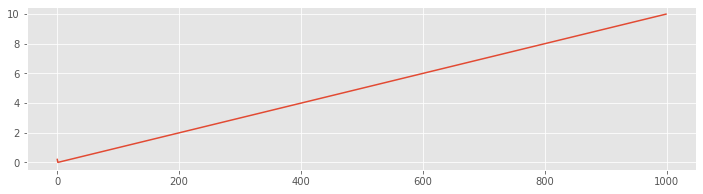
Q: What happens to the voltage after 1000 steps?
This plot is informative, but not great. Really, we’d like to plot the voltage as a function of time, not steps or indices. To do so, we need to define a time axis:
t = arange(0,len(V))*dt
Q: What’s happening in the command above? Does it make sense? (If not, trying printing or plotting t.)
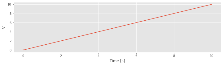
Now, with time defined, let’s redo the plot of the voltage with the axes labeled appropriately.
figure()
plot(t,V)
xlabel('Time [s]');
ylabel('V');
Finally, let’s put it all together …
Part 3: I&F CODE (version 1)
In Parts 1 and 2, we constructed parts of the I&F model in bits-and-pieces. Let’s now collect all of this code, compute a numerical solution to the I&F model, and plot the results (with appropriate axes).
First, let’s clear all the variables:
%reset
from pylab import *
%matplotlib inline
rcParams['figure.figsize']=(12,3)# Change the default figure size

I=1                              #Set the parameter I.
C=1                              #Set the parameter C.
dt=0.01                          #Set the timestep.
V = zeros([1000,1])              #Initialize V.
V[0]=0.2;                        #Set the initial value of V.

for k in range(1,999):           #March forward in time,
    V[k+1] = V[k] + dt*(I/C)     #... updating V along the way.

t = arange(0,len(V))*dt          #Define the time axis.

figure()                         #Plot the results.
plot(t,V)
xlabel('Time [s]')
ylabel('Voltage [mV]');
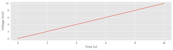
Q: Adjust the parameter I. What happens to V if I=0? Can you set I so that V > 20 within 10 s?
Part 4: Voltage threshold
Notice, our model is missing something important: the reset. Without the reset, the voltage increases forever (if \(I>0\)). Now, let’s update our model to include the reset. To do so, we’ll need to add two things to our code.
First, we’ll define the voltage threshold
Vth, and reset voltageVreset.Second, we’ll check to see if
VexceedsVthusing an if-statement; if it does, then we’ll setVequal toVreset.
Here’s what we’ll add to the code:
Vth = 1;        #Define the voltage threshold.
Vreset = 0;     #Define the reset voltage.

for k in range(1,999):            #March forward in time,
    V[k+1] = V[k] + dt*(I/C)      #Update the voltage,
    if V[k+1] > Vth:              #... and check if the voltage exceeds the threshold.
        V[k+1] = Vreset
Part 5: I&F CODE (version 2)
Now, let’s put it all together to make a complete I&F model (with a thershold and reset), simulate it, and plot the result.
%reset
from pylab import *
%matplotlib inline
rcParams['figure.figsize']=(12,3) # Change the default figure size

I=1                          #Set the parameter I.
C=1                          #Set the parameter C.
Vth = 1;                     #Define the voltage threshold.
Vreset = 0;                  #Define the reset voltage.
dt=0.01                      #Set the timestep.
V = zeros([1000,1])          #Initialize V.
V[0]=0.2;                    #Set the initial condition.

for k in range(1,999):       #March forward in time,
    V[k+1] = V[k] + dt*(I/C) #Update the voltage,
    if V[k+1] > Vth:         #... and check if the voltage exceeds the threshold.
        V[k+1] = Vreset

t = arange(0,len(V))*dt      #Define the time axis.

figure()                     #Plot the results.
plot(t,V)
xlabel('Time [s]')
ylabel('Voltage [mV]');
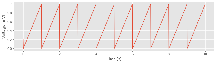
Q: Adjust the parameter I. What happens to V if I=10? If I=100?
Q: Adjust the parameter C. What happens to V if C=0.1? If C=10?
Q: What is “spiking” in this I&F model?