Reproducible exploratory analysis - Mitigating multiplicity when mining data
Identifying meaningful patterns and relationships within noisy data is a fundamental component of neuroscience research; however, multiplicity—the practice of conducting multiple simultaneous comparisons—can result in spurious and misleading conclusions. By contrast, overly strict corrections for multiplicity can cause us to miss meaningful scientific conclusions. In this unit, learners will understand how multiplicity occurs, its impacts, and strategies to address it.
0. Why mitigate multiplicity?
In science, it’s common to test data in multiple ways. We might use our data to test multiple theories or we might test multiple features of data collected from a novel device.
After doing so, we often want to make confident statements about these test results. It’s then important to deal with the challenges of multiplicity. Multiplicity occurs whenever we have multiple opportunities to find a result. The more tests we perform, the more likely we are to obtain at least one apparently meaningful result purely by chance - even when no real effect exists.
For example:
- A researcher tests whether a treatment affects 20 different health outcomes.
- A geneticist tests thousands of genes to determine which are associated with a disease.
- A researcher examines several subgroups, outcomes, and time periods, then reports the most promising result.
In each case, performing more tests creates more opportunities for chance findings.
After performing these tests, we often want to make confident statements about the results. It is therefore important to address the challenges created by multiplicity.
There are at least two common mistakes when confronting multiplicity:
Too lenient. If we do nothing about multiplicity in our results, then we might mistake spurious results occurring by chance for meaningful scientific findings.
Too strict. If we too aggressively address multiplicity, then - in our quest to avoid false positive results - we might overlook real and meaningful scientific conclusions.
Unfortunately, no one-size-fits-all solution exists to address multiplicity. The appropriate approach depends on the scientific question, the number and structure of the tests, and the consequences of false-positive and false-negative conclusions.
Our goal in this unit is to practice making decisions about multiplicity and to explore the consequences of being too lenient or too strict.
1. Rat brains, position, and profit: an introduction to mitigating multiplicity
The first suspicious scenario
Consider the following data mining scenario:
A research group inserts tiny electrodes into a rodent brain and records the activity of individual neurons while the rat performs 5 behaviors: walks, eats, drinks, grooms, and sleeps.
The researchers collect data from the 76 neurons and 5 behaviors and then choose 8 neurons to analyze.
The researchers report observations from a handful of observations from the selected 8 neurons, such as how different neurons respond (i.e., generate action potentials) during some of the rat’s different behaviors (e.g., during walking, or during grooming).
A second suspicious scenario
Consider this press release from another data mining scenario:
EXTRA! EXTRA! RAT BRAINS CRACK THE STOCK MARKET CODE!
In a dazzling demonstration of rodent ingenuity—or perhaps sheer luck—researchers have harnessed the firing neurons of rat motor cortices to predict movements in the U.S. stock market. That’s right, folks! A team from Michigan and Georgia linked rat brain activity to Wall Street ticker tapes, proving that whiskers may rival Wall Street wits. By monitoring the firing rates of 94 neurons across three rats, these scientists uncovered correlations between neural activity and the daily closing prices of 4195 stocks on NASDAQ, the NYSE, and the American Stock Exchange. The Coca-Cola stock price, for instance, danced in sync with the neurons like Fred and Ginger at the Ziegfeld Follies.
But wait, there’s more! The researchers didn’t stop at finding patterns — they dove headfirst into the trading floor with a predictive model based on neural firing rates. Rats’ neural spikes gave the orders: buy, sell, or hold. And the results? An impressive 43% increase in a simulated portfolio value, turning an initial $1,000 investment into a snappy $1,435 over just 20 trading days. Forget the contrarian strategies of hedge fund honchos—our furry friends seem to have cracked the code.
And here’s the kicker, folks: this isn’t just about making a buck. The findings suggest a mysterious connection between rat neural activity and human economic behavior. The researchers propose a grand theory linking the creatures of Earth to the ebbs and flows of societal urges, tying their work to theories like Gaia’s interconnected organism hypothesis. So, the next time someone says, “it’s a rat race out there,” remember—they might just be running the show!
So, what do we believe?
Using noisy data recorded from rodent brains, the two scenarios above report relationships between:
the brain’s neural activity and rodent behavior, and
the brain’s neural activity and the stock market prices.
You might be (reasonably) skeptical. How could neural activity from a rat brain possibly predict so many different things?
In what follows, we’ll investigate this question with the goal of confronting the challenge of multiplicity.
N neurons (e.g., spiking activity) and M signals (e.g., stock prices). How many possible combinations of relationships exist between the neurons and signals?
2. Does this really work? Analyze some data
Motivated by these previous scenarios, you receive data from a collaborator interested in understanding the relationship between neural activity in the rodent brain, measures of rodent behaviors (e.g., measures of the rodent’s position, movement speed, head angle, etc.), and stock prices on the NYSE. The data consist of the following information:
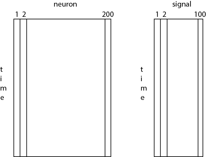
spikes- the action potentials (or “spikes”) generated by 200 neurons,signals- rodent behaviors (10 of the signals) and the price of 90 stocks.
Both the spikes and signals are recorded simultaneously, every 1 ms for 0.5 s, resulting in a total of 500 data points.
We’re interested in understanding the relationship (if any) between spikes and signals.
Let’s start by investigating the structure of the data.
Both spikes and signals consist of 500 time points (the number of rows). We collect data from 200 neurons and 100 signals (the number of columns).
You might think of these variables as rectangles (or matrices), where each row indicates a time point, and each column indicates a neuron or signal:
Let’s plot the data from one neuron in spikes:
spikes?
Let’s also plot the data from one signal in signals:
signals?
To more directly compare the spikes and signals, let’s plot one atop the other:
spikes) and one signal (the first column of signals). We didn’t see an obvious relationship. However, there are many more relationships to compare. Repeat this analysis to compare each spike train (all 200 columns of spikes) with each signal (all 100 columns signals). Do you observe any relationships?
Alert: We can’t use visualization alone!
There are 200 neurons and 100 signals, resulting in 20,000 pairs to consider.
We can’t possibly visualize all of those.
Instead, we need to perform statistical tests.
3. Profit! Rat brains for high-frequency trading on the NYSE
Let’s now investigate the pairwise associations between the spiking of 200 neurons in the rat brain with signals related to rat behavior and stock prices.
To compare the spikes and signals, we perform a statistical test of the association between each pair of variables. There are many choices you could make to assess the associations and perform the statistical tests. We will not investigate those choices here. Instead, we will use a sophisticated—yet standard—approach to assess the relationship between the spikes and signals; if you’re interested in (many) more analysis details, check out this link.
Again, for our purposes, the details of the test are not important.
What is important is that each test produces a p-value and we interpret small p-values to indicate statistically significant associations (Putting the p-value in Context).
Let’s compute those p-values now.
This step is slow, because there are many p-values to compute!
For each neuron-signal pair, we estimate the association and its p-value.
We now have 20,000 p-values to investigate.
To start, let’s visualize those p-values.
To isolate meaningful relationships, let’s count the number of associations in which \(p < 0.05\), a standard threshold for significance applied in practice (see Putting the p-value in Context).
Conclusion:
- We detect many significant associations between rat brain neural activity, stock prices, and the rodent’s position!
- Let’s develop a new strategy for profitable high-frequency stock trading using rat brain neuron spiking.
Reflection:
- Hmm, there are a lot of significant relationships - this was so easy!
- Why doesn’t everyone use rat brain activity to predict the stock market?
Alert: Wait, this doesn’t make sense!
How can the spike timing in a rat brain relate to stock market prices?
We’ve conducted many (20,000 in fact) statistical tests and identified all associations with p<0.05
… Is that the right choice?
4. Not so fast … finding meaningful relationships after you’ve tested everything.
In the previous section, we assessed associations between 200 neurons and 100 signals.
This exploration led to many (20,000) statistical tests.
When we compute so many tests, we need to correct for multiplicity.
Important fact: When conducting multiple hypothesis tests, increased error rates occur because each test has a chance of incorrectly rejecting the null hypothesis (a false positive). This error, typically called the Type I error, is the probability of a single test falsely claiming a statistically significant effect.
As more tests are performed, the cumulative probability of committing at least one Type I error across all these tests increases, leading to an overall higher error rate for the set of tests than for any individual test. This phenomenon is often referred to as the “multiple comparisons problem” or “multiplicity.”
To mitigate multiplicity in our analysis, we must account for increased error rates due to conducting multiple hypothesis tests on the same dataset.
Intuition building aside
Imagine you have a fair coin and you flip it 5 times. Let’s think about what happens.
Now, back to the main story - the Bonferroni correction
Many methods exist to correct for multiplicity. In this unit, we’ll investigate three of these methods.
To start, let’s apply one of the most popular procedures to correct for multiplicity: the Bonferroni correction.
The Bonferroni correction reduces the Type I error rate by dividing the desired overall significance level (\(\alpha\)) by the number of tests performed (call it \(m\)). For example, if a trial is testing \(m = 20\) hypotheses with a desired overall \(\alpha = 0.05\), then the Bonferroni correction would test each individual hypothesis at \(\alpha = 0.05/20 = 0.0025\).
The Bonferroni correction is considered conservative because it adjusts the significance level \(\alpha\) by dividing it by the number of comparisons. Doing so reduces the risk of Type I errors (false positives) but increases the likelihood of false negatives (i.e., incorrectly labeling a significant relationship as not significant).
signals and spikes data, compute the Bonferroni adjusted significance level using our desired overall significance level (\(\alpha = 0.05\)) and the number of tests performed.
Let’s apply the Bonferroni correction to our matrix of p-values (p) and determine the number of significant associations, after correcting for multiplicity.
Alert: Wait, this doesn’t make sense!
Much work (including Nobel Prize work) has established a relationship between rat neuron spiking and rodent position.
We’ve identified all associations with \(p < 0.05 / 20000\) after Bonferroni correction … and there aren’t any.
Is that the right choice?
5. Rat brains either predict many things or no things?
We’ve applied two strategies to confront multiplicity in our analysis:
The two strategies give completely different results. When we do nothing (Part 3), we conclude that neurons in the rat brain spike in association with many observed signals, including rodent behavior and stock prices. However, when we correct for multiplicity using the Bonferroni correction (Part 4), we identify no associations between signals and spikes. Neither result makes sense when compared to the existing literature.
So, now what?
Again, many strategies exist to correct for multiplicity. There’s no single “right” approach.
Our first approach (do nothing) is too lenient - we allow too many false positives. And, in doing so, we draw a ridiculous scientific conclusion: action potentials in the rat brain predict prices on the stock market.
Our second approach (Bonferroni correction) is too strict - we allow too few false positives. And, in doing so, we find no evidence for a well-established scientific conclusion: action potentials in the rat brain encode the rodent’s position.
Perhaps we can find an intermediate approach, that allows neither too many nor too few false positives …
In what follows, we’ll implement alternatives to our choices above, and see how these choices to address multiplicity impact our results.
6. FDR: a less conservative approach to multiplicity.
We’ll first consider a popular choice to mitigate the impact of performing multiple statistical tests: calculate the False Discovery Rate (FDR).
To do so, we’ll use the Benjamini-Hochberg (BH) procedure. The BH procedure is a statistical method to control the false discovery rate (FDR) in multiple hypothesis testing. It ranks the p-values from smallest to largest and compares each to a threshold that increases with rank, defined as \((r/m) \cdot q\), where \(r\) is the rank of the p-value (i.e., the p-value’s position when ordered from smallest to largest), \(m\) is the total number of tests, and \(q\) is the desired FDR level, which is the expected proportion of false positives among all rejected hypotheses. For example, if \(q = 0.05\), it means that, on average, no more than 5% of the rejected hypotheses are expected to be false positives. This allows for a controlled balance between identifying true effects and limiting false discoveries in multiple hypothesis testing.
The BH procedure is less conservative than methods like Bonferroni correction, offering more power while maintaining control over the expected proportion of false positives.
The BH procedure is implemented in three steps:
Assign each p-value a rank, \(r\), where the smallest p-value has rank \(r=1\), the next smallest has rank \(r=2\), and so on.
Calculate the critical value for each rank \(r\) using the formula:
\(CriticalValue =(r/m) \cdot q\)
where \(m\) is the total number of tests, and \(q\) is the desired overall significance level (typically 0.05 for 5% FDR).
- Compare each p-value to its corresponding critical value. The largest rank, \(r\), for which the p-value is less than or equal to the critical value is considered significant, and all p-values with ranks less than or equal to this \(r\) are considered significant. In other words, we reject the null hypothesis for all p-values with ranks less than or equal to \(r\).
To build some intuition for these steps, let’s start with a simple example.
Consider an experiment in which you perform 5 hypothesis tests (\(m=5\)) and collect 5 p-values:
p-value: [0.1, 0.12, 0.001, 0.015, 0.045]
We conducted 5 tests and decided to correct for multiplicity.
Let’s use the p-values to perform each step of the Benjamini-Hochberg procedure.
Example - Step 1. Assign each p-value a rank.
Example - Step 2. Calculate the critical value for each rank.
Example - Step 3. Compare each p-value to its corresponding critical value.
Now, back to the main story.
Having built some intuition for computing the FDR using the Benjamini-Hochberg (BH) procedure, let’s apply it to our data of interest.
It’s the same idea, but instead of considering 5 p-values as we did in the simple example, we must consider the 20,000 p-values.
The function fdr returns whether each p-value in p remains significant after correcting for multiplicity using FDR.
Let’s display the p-values that remain significant after correcting for multiplicity using FDR.
Interpretation:
We originally corrected for multiplicity using the Bonferroni correction. Following this strict correction, we found no evidence of significant associations between
spikesandsignals.After correcting for multiplicity using FDR, we now find some neurons in the rat brain are associated with some signals.
We return to our collaborators, and they confirm that signals 0-10 correspond to different measures of the rodent’s behavior.
Relief
We’ve corrected for multiple comparisons using FDR and find a sensible result.
The results are consistent with the existing theory that neurons in the brain encode rodent position.
We find no evidence that neurons in the rodent brain predict stock market prices.
Using a less strict correction (FDR instead of Bonferroni), we identify significant associations in the data.
7. Split the Data
Splitting the data means exactly what it says: we’ll split the data into two halves. In the first half of the data, we’ll perform an exploratory analysis and identify significant relationships between spikes and signals. Then, we will test those identified relationships in the second half of the data.
This process of “splitting the data” is more formally called a split-sample screening/validation procedure.
Let’s do it.
We’ll split the data in time; for the first half of the data, we’ll consider all neurons and all signals from the first 0.25 s of the recording. We do so because we want to assess the relationships between all neurons and all signals. We’ll do so using the first half of our observations.
Because we’ve computed so many p-values (200 neurons * 100 signals = 20,000 p-values), we expect to find p<0.05 by chance. We must mitigate this multiplicity!
Let’s determine the number of significant associations in the first half of the data, without (yet) correcting for multiplicity.
We find 981 associations with \(p < 0.05\). This is not surprising, because with 200 neurons and 100 signals, we expect about \[ 200 * 100 * 0.05 = 1000 \] false-positive detections to occur by chance.
But, we’re not done yet.
Our next step is to test these associations in the second half of the data.
Note that we no longer test all possible associations between the 200 neurons and 100 signals. Instead, we restrict our analysis to the subset of associations identified as significant (\(p < 0.05\)) in the first half of the data.
Doing so, we dramatically limit the number of tests we’ll perform in the second half of the data.
Instead of the 20,000 tests we performed in the first half of the data, we’ll perform 981 statistical tests in the second half of the data.
Finally, to correct for multiplicity (we did still perform almost 1000 tests), let’s apply FDR correction to these p-values.
We find that three significant associations remain.
Let’s visualize these validated associations.
Interpretation:
We originally corrected for multiplicity using the Bonferroni correction. Following this strict correction, we found no evidence of significant associations between
spikesandsignals.We now split the data to correct for multiplicity. In our first split, we performed 20,000 tests and identified 981 associations with \(p<0.05\). We then tested this subset of associations in the second split, and corrected for multplicity using FDR.
After splitting, we find some neurons in the rat brain are associated with some signals.
We return to our collaborators, and they confirm that signals 0-10 correspond to different measures of the rodent’s behavior.
Relief
We’ve corrected for multiple comparisons by splitting our data and find a sensible result.
The results are consistent with the existing theory that neurons in the brain encode rodent position.
We find no evidence that neurons in the rodent brain predict stock market prices.
Using a less strict correction (splitting instead of Bonferroni), we identify significant associations in the data.
Q. When would you not use splitting to account for multiplicity in your data? A. When the data change in time (i.e., the second half of data is meaningfully different than the first) (correct) When the associations differ among spikes When the associations differ among signals When the associations differ among spikes and signals
8. Conclusions
Exploratory analysis allows us to discover patterns in noisy data. But, when we test many possible relationships, we create a rigor problem: some results will appear significant by chance. In our example dataset, 20,000 tests at \(\alpha = 0.05\) would produce approximately 1000 false positives if all of the null hypotheses were true.
We applied four approaches to address the problem of multiplicity in these data.
Do nothing: This approach was too lenient. We found apparent relationships between rat brain activity and stock prices, but most of the 1104 results with
p < 0.05could occur by chance.Apply the Bonferroni correction: This approach controlled the probability of making any false-positive claim, but it was too strict for these data. We found no significant associations, including no evidence for the well-established relationship between neural activity and rodent position.
Control the False Discovery Rate: The Benjamini-Hochberg procedure accepts a controlled proportion of false discoveries in exchange for greater power. It recovered associations between neural activity and rodent position and none with stock prices.
Split the data: The first half of the data generated candidate relationships, and the second half tested them. This separation of exploration from validation left three significant associations, all involving measures of rodent position.
The rat-brain stock-market study was intentionally tongue-in-cheek satire. Its ridiculous conclusion nevertheless illustrates a real threat to rigor: if we search enough unrelated signals and report only the most interesting results, chance associations can tell a compelling story. A rigorous report should make the exploratory nature of the analysis clear, describe how many relationships were tested, report nonsignificant as well as significant results, and explain how multiplicity was addressed.
The early rodent-position study sits in a different scientific context. From a modern perspective, selecting 8 neurons from 76 and reporting a handful of relationships raises reasonable questions: How were those neurons and behaviors selected? How many relationships were examined? Yet that exploratory work contributed to a finding that was supported by converging evidence and eventually recognized with a Nobel Prize. The lesson is not that exploratory analysis is unscientific. Exploratory results can generate transformative hypotheses, but confidence grows when those results are transparently reported, replicated, and supported by independent evidence.
Correcting for multiplicity is therefore one part of rigorous scientific inference, not a complete solution. Other strategies developed across these units also matter: choose an adequate sample size, interpret p-values in context, and repeatedly check and refine the inference model.