Putting the p-value in Context

Neuroscience researchers typically report p-values to express the strength of statistical evidence; but p-values are not sufficient on their own to understand the meaning and value of a scientific inference. In this unit, learners will learn how to interpret the p-value, how to express the size of an effect and uncertainty about a result, and how to interpret results at both the individual and population levels.

1 - You want to do some science; your PI just wants the p’s!

Introduction

• You work in a sleep lab studying the effect of a new treatment regimen on memory consolidation during sleep.

• Your lab collects an EEG biomarker of memory (sleep spindles) from N=20 human subjects.

• To do so, your lab measures the power in the spindle band (9-15 Hz) twice per minute. Your lab has a reliable method to detect spindle activity; this detector is known to have small measurement errors outside of treatment. You expect it to still work during treatment, but also expect more variability in the spindle power estimates (hence more variability in the detections) during treatment.

• For each subject, your lab measures spindle activity during three conditions:

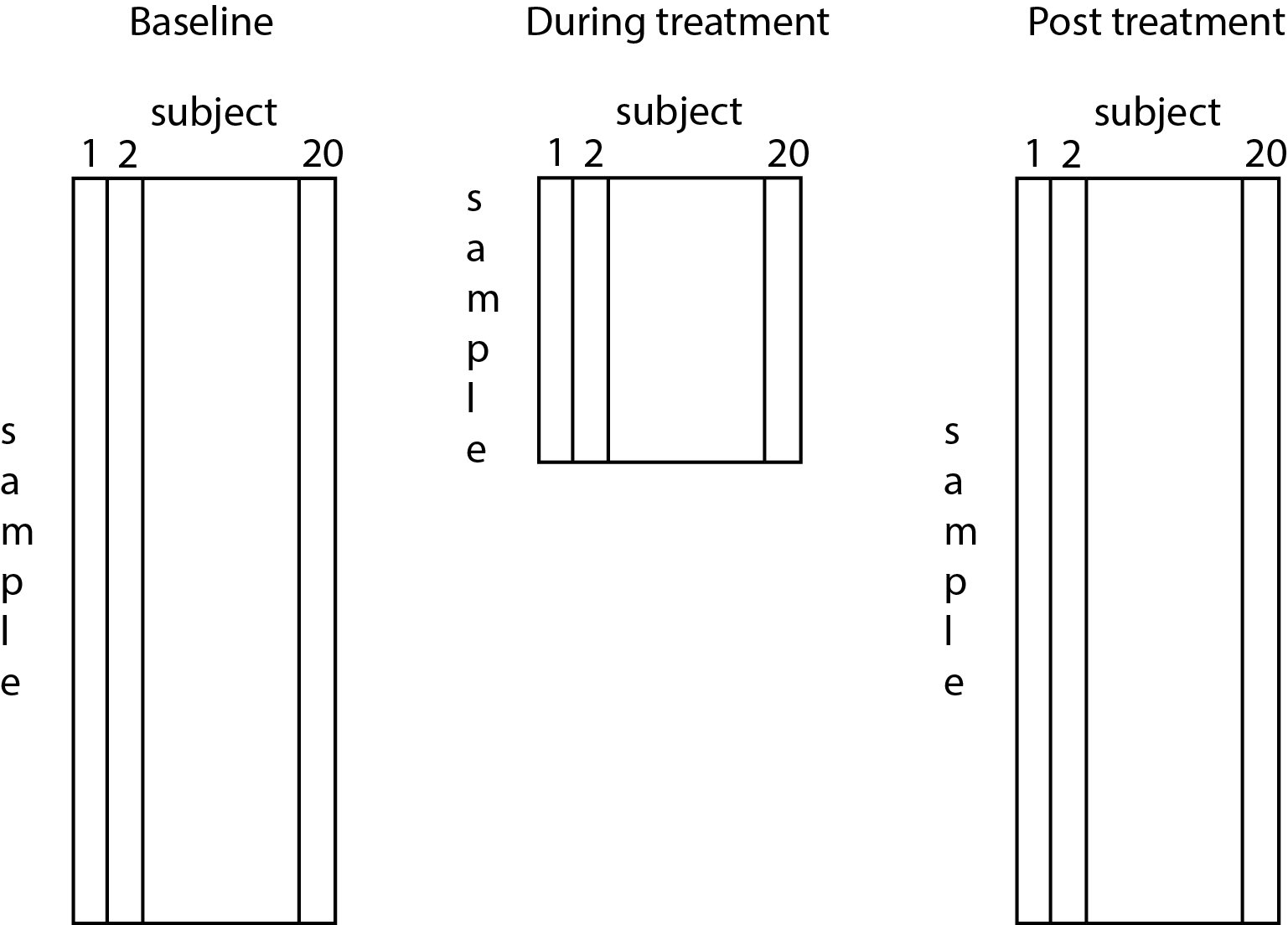
  • Baseline: Data collection lasts 7 hours while the subject sleeps the night before the intervention. This results in 840 samples of spindle activity for each subject.

  • During Treatment: Data collection during a 15 minute intervention during sleep, resulting in 30 samples of spindle activity for each subject.

  • Post-treatment: Data collection after intervention lasts 7 hours, while the subject sleeps, resulting in 840 samples of spindle activity for each subject.

Here’s a graphical representation of the data collected from one subject:

Your PI says: “I hypothesize that some subjects will show an increase in spindle activity as a result of this treatment. Other subjects may not respond to the treatment. Conduct a hypothesis test for each subject to determine if they are responsive and report the p-values associated with each test.”

What information would the p-values associated with these hypothesis tests provide?

The p-values indicate which subjects show an increase in spindle activity as a result of treatment.
The p-values indicate subjects who are more likely to show an increase in spindle activity if the treatment were applied again.
The p-values indicate subjects for whom the null hypothesis that treatment has no effect is probably false.
The p-values indicate subjects for whom the effect of the treatment was large enough to be of scientific significance.
The p-values indicate the probability under a specific statistical model that a selected statistic would be equal to or more extreme than its observed value if treatment does not have an effect on spindle activity.

Fundamentally, p-values indicate how incompatible a data set is with a specified statistical model, but they do not express a probability that any scientific hypothesis is correct or whether on hypothesis is more likely true than another. P-values can be part of a strong statistical argument, but do not provide a robust measure of evidence about a hypothesis on their own. In particular, a p-value needs to be paired with a measure of effect size to describe whether an effect is scientifically meaningful.

Another important issue is that p-values are often only meaningful in cases where the scientific question to answer has only a binary outcome. Most scientific questions require more than yes or no answers, but it is common to see researchers try to shoehorn their experiments to produce binary outcomes just so that they can express their results using p-values. This risks throwing away useful information and decreasing the statistical power of an argument.

For each scenario, is it most appropriate to use a p-value?

1. Does the proportion of people who prefer brand A over brand B differ from 50%?
   Yes No



2. What is the exact average height of an adult giraffe in meters?
   Yes No



3. Does a new vaccine significantly reduce infection rates compared to the old vaccine?
   Yes No



4. How long does it take to completely drain a 50,000-gallon swimming pool?
   Yes No



5. Does changing the color of a website’s button increase user clicks statistically significantly?
   Yes No

Discussion

Based on your understanding of how to interpret p-values, are there any concerns about your PIs analysis plan to just report p-values for separate tests conducted on each subject? What other approaches could you use to evaluate the effect of treatment in the subject population?

At this point, perhaps you feel that we should just get rid of p-values entirely. Good idea! Many researchers and statisticians agree with you. But despite multiple organized efforts to downplay the use of p-values in scientific research, a focus on computing and reporting p-values has persisted.

You have a detailed discussion with your PI about the issues with focusing on p-values for this study, but your PI says: “We’re not going to be able to publish anything unless we show statistical significance so just give me the p’s!”

---

2- Let’s do it: Define & compute p-values.

Before we compute p-values, let’s consider what a p-value means.

What does a p-value mean?

A p-value is used to compare two competing hypotheses. If our scientific hypothesis is that spindle activity changes during treatment relative to its baseline level of activity, we need another hypothesis to compare this to. In this case, we can hypothesize that the spindle activity does not change during treatment. This is called the null hypothesis.

Our goal is to collect data that provides evidence in favor of our scientific hypothesis over the null hypothesis. But this is not a fair fight; we start by assuming that the null hypothesis is true and only reject it after we achieve a sufficiently high bar of evidence. The p-value tells us how high a bar we have achieved.

One useful analogy is proof by contradiction. There, we assume that a hypothesis is true and show that this assumption leads to a contraction. If we were to observe data that could not possibly occur if the null hypothesis were true, this would be definitive evidence against that hypothesis. However, it is not the case that if we observe data that is unlikely if the null hypothesis were true then the null hypothesis is itself unlikely.

For example, most people would agree with the following statement, “If a person is American, they probably are not the US President.” Now imagine that we select an individual at random and they happen to be the US President. It is clearly not the case that this individual is probably not American. While the observation that this individual is the US president is unlikely under the null hypothesis that this individual is American, it is much more unlikely (or impossible) under the alternate hypothesis that they are not American.

Another useful analogy is to a prosecutor at a trial. In this analogy, the null hypothesis is akin to the hypothesis that the defendant is innocent. The court assumes that defendant is innocent until proven guilty. The prosecutor tries to amass and present evidence to demonstrate that the defendant is guilty beyond a reasonable doubt. A strong argument needs to include evidence that would be unlikely to occur if the hypothesis that the defendant is innocent is true, and more likely to occur if the hypothesis that the defendant is guilty is true. If the prosecutor fails to provide sufficient evidence that the defendant is guilty, it doesn’t necessarily mean that they are innocent.

In a statistical test, the p-value indicates how surprising our evidence would be if the null hypothesis were true. For our problem, if we’re sufficiently surprised by the observed data, then we’ll reject the null hypothesis, and conclude that we have evidence that the spindle activity changes relative to baseline.

Alternatively, if we’re not surprised by the observed data, then we’ll conclude that we lack sufficient evidence to reject the null hypothesis. There’s an important subtlety here that statisicians like to point out - when we’re testing this way, we never accept the null hypothesis. Instead, the best we can do is talk like a statistician and say things like “We fail to reject the null hypothesis”. In our court analogy, this is equivalent to finding the defendant not guilty rather than innocent, because we realize that it is possible that defendant committed the crime but we lacked the evidence to convince a jury beyond a reasonable doubt.

Multiple factors impact the evidence we have to reject a null hypothesis. In this Unit, we’ll explore these factors and how they influence the p-values we compute.

The PI says: “I expect that during treatment the spindle activity exceeds the baseline spindle activity.” What is the null hypothesis?

The average spindle activity during treatment is guaranteed to be higher than baseline.
The average spindle activity during treatment is guaranteed to be lower than baseline.
A difference in average spindle activity exists between treatment and baseline.
No difference in average spindle activity exists between treatment and baseline.

What does p<0.05 mean?

The probability of observing the data, or something more extreme, under the null hypothesis is less than 5%. This is typically considered sufficient evidence to reject the null hypothesis in favor of the alternative hypothesis (which posits that there is an effect or a difference). In other words, a p-value less than 0.05 suggests that the observed data is unlikely to have occurred by random chance alone, assuming the null hypothesis is true, leading researchers to reject the null hypothesis.

In our case, the null hypothesis we will first investigate is:

Null hypothesis: No difference in average spindle activity between treatment and baseline conditions.

Which of the following factors might impact the evidence you have to reject this null hypothesis?

(Select all that apply)

Sample Size: Collecting more spindle samples reduces random error and provides more precise estimates.
Effect Size: Bigger differences in spindle activity between conditions are easier to detect.
Variability (or Noise) in Measurements: High variability in the spindle estimates during treatment can make it harder to detect a real effect.

Now, let’s load the spindle data and compute p-values to test our null hypothesis

Let’s start by investigating the structure of the data.

All three variables consist of observations from 20 subjects (the number of columns).

During baseline: We collect 840 samples per subject.

During treatment: We collect 30 samples per subject.

After treatment: We collect 840 samples per subject.

The number of samples is the number of rows for each variable.

You might think of these variables as rectangles (or matrices) - each row indicates a sample of spindle activity, and each column indicates a subject:

Look at the representations of the data above. What differs about the data during treatment, compared to baseline and post-treatment?

There are fewer subjects during treatment.
There are fewer samples during treatment.

To get a sense for the the data, let’s plot the spindle activity during baseline, treatment, and post-treatment conditions for one subject:

What values do you observe for the spindle activity?

The values are always positive.
The values are always negative.
The values stay constant at zero.
The values tend to fluctuate around 0 and can be both positive and negative.

Here, the spindle activity has been z-scored during each recording interval relative to baseline.

So, the values we observe indicate changes relative to the mean baseline spindle activity.

Positive (negative) values indicate increases (decreases) in spindle activity relative to the baseline activity.

What differences or similarities do you notice in spindle activity during the baseline, treatment, and post‐treatment conditions for this subject?

All three conditions have the same number of samples and similar fluctuation sizes.
Only baseline and post‐treatment fluctuate around zero; treatment values stay positive.
Treatment has more samples than baseline and post‐treatment, with smaller fluctuations.
All conditions fluctuate around zero; during treatment there are fewer samples and larger fluctuations (greater variability).

During treatment, we collect fewer, noisier samples compared to the baseline and post‐treatment conditions. How might these factors impact the evidence we have to reject the null hypothesis?

Null hypothesis: No difference in average spindle activity between treatment and baseline conditions.

Fewer spindle samples increases our evidence.
Fewer spindle samples decreases our evidence.
Noisier spindle samples increases our evidence.
Noisier spindle samples decreases our evidence.

Is there a significant effect treatment? Let’s now compute some p-values.

To do so, we again assume the null hypothesis:

Null hypothesis: No difference in average spindle activity between treatment and baseline conditions.

To test this hypothesis, we’ll compute a two-sample t-test.

The two-sample t-test is by far the most popular choice when comparing two distribution.

We use this method method used to determine if there’s a significant difference between the means of two independent groups. It’s commonly applied to compare the average values of (continuous) variables across two different populations or conditions.

In our case, we’d like to compare the average spindle activity between treatment and baseline conditions. So, the two-sample t-test is (at first glance) a completely reasonable approach.

The list above consists of 20 p-values, one for each subject.

Each p-value indicates the probability of observing the data, or something more extreme, under the null hypothesis:

Null hypothesis: No difference in average spindle activity between treatment and baseline conditions.

Let’s print the p-values for each subject:

For Subject 0, we find p = 0.52. What does this mean?

There is a 52% chance that the mean spindle rate is truly zero.
There is a 52% probability of observing these data (or something more extreme) if the mean spindle rate is zero.
There is a 48% probability that the alternative hypothesis is correct.
There is a 52% chance that the result is clinically meaningful.

Let’s also plot the p-values:

Interpret the print‐out and plots of p‐values. What do you see?

Most p‐values are below 0.05, indicating significant effects across subjects.
The p‐values tend to exceed 0.05 (red dashed line), although a few subjects have p < 0.05.
All p‐values cluster exactly at the threshold, suggesting borderline significance.
The p‐values form a uniform distribution from 0 to 1, indicating no pattern in the data.

Do we have evidence to reject the null hypothesis?

Maybe … if we had performed one statistical test, then we typically reject the null hypothesis if

p < 0.05

But here we compute 20 test (one for each subject).

When we perform multiple tests, it’s important we consider the impact of multiple comparisons. We cover this topic in detail in the Multiplicity Unit.

Here we’ll chose a specific approach to deal with multiplicity - we’ll apply a Bonferroni correction. The Bonferroni correction reduces the Type I error rate by dividing the desired overall significance level (here 0.05) by the number of tests performed (here 20 tests, one test per subject). Stated simply, the Bonferroni test adjusts the significance level by dividing it by the number of tests we perform. Doing so reduces the risk of false positives (Type I errors); or more information, see Multiplicity Unit.

So, for our analysis of the p-values from 20 subjects, let’s compare the p-values to a stricter threshold of

p < 0.05 / 20 or p < 0.0025

Thresholding in this way provides a binary, yes/no answer to the question: do we have evidence that the spindle activity during treatment differs from 0?

Let’s plot the p-values versus this new threhsold.

After the Bonferroni correction, can we reject the null hypothesis for any subject?

No. None of the p-values are less than 0.05/20.
Yes. Some of the p-values are small enough.

The PI requested “Give me the p’s!”. Do you have evidence to reject the null hypothesis during treatment?

No! The p-values are large, so we find no evidence to reject the null hypothesis for any subject.
Yes! The p-values are large, so the spindle activity during treatment is large.

We do not find any p-values that pass our significance threshold during treatment. Does this mean that the spindle activity during treatment does not change relative to baseline?

No! We never accept the null hypothesis. Instead, we say: “We fail to reject the null hypothesis that the spindle activity during treatment differs from baseline.”
Yes! Because the p-values are large, we can accept the null hypothesis.

Summary:

We’ve computed a p-value for each subject. After correcting for multiple comparisons, our intial results suggest no evidence that we can reject the null hypothesis (of no difference in spindle activity between baseline and treatment).

Mini Summary & Review

We sought to answer the scientific question:

• Does the spindle activity during treatment differ from the baseline spindle activity?

To answer this question, we assumed a null hypothesis:

Null hypothesis: No difference in average spindle activity between treatment and baseline conditions.

We tested this null hypothesis for each subject, computing a p-value for each subject.

Because we computed 20 p-values (one for each subject), we corrected for multiple comparsions using a Bonferroni correction (see Multiplicity Unit).

We found no p-values small enough to reject the null hypothesis.

In other words, using our initial approach, we found no evidence that the spindle activity during treatment differs from baseline.

Our initial results show no evidence that spindle activity during treatment differs from baseline. What factors might impact our evidence?

(Select all that apply)

Sample Size: We collect only 30 spindle samples during treatment, which increases random error and provides less precise estimates.
Effect Size: Small differences in spindle activity between conditions are difficult to detect.
Variability (or Noise) in Measurements: High variability in the spindle estimates during treatment can make it harder to detect a real effect.
Approach to Statistical Testing: A different approach may provide more insight into differences in spindle activity between treatment and baseline.
Treatment has no Effect: It may be that the treatment does not impact spindle activity relative to baseline.

---

3- Maybe there’s something else we can publish?

Our initial results are discouraging; we find no evidence of a change in spindle activity from baseline during treatment.

That’s dissappointing. Rather than abandon our data (which took years to collect), our PI asks us to continue exploring the data.

Data exploration is common in neuroscience. In general, as practicing neuroscientists, we explore our data for interesting features.

However, when undertaking data exploration, we must make it clear (e.g., by reporting what we explored, whether the results are significant or not).

Our PI recommends that we examine the change in spindle activity post-treatment.

Perhaps the treatment produces a longer-term affect that manifests during the post-treatment period.

Exploratory vs Confirmatory Analyses & Guarding Against p-Hacking

Our initial results are discouraging: we find no evidence of a change in spindle activity from baseline during treatment.

Instead of discarding years of data, our PI encourages us to explore the data for unexpected patterns — this is perfectly legitimate as long as we remain transparent.

• Data exploration helps generate new hypotheses. We might notice trends, outliers, or condition-specific features that suggest where real effects could lie, to help guide future experiments.

• P-hacking occurs when we repeatedly mine the data—trying different subsets, covariates, or outcomes—until something “significant” emerges. This inflates false positives and misleads follow-up studies.

• To stay honest, every exploratory analysis must be clearly labeled as such. We should report exactly what we tested (e.g. “we examined spindle rate in the baseline, treatment, and post-treatment intervals), and include both significant and nonsignificant findings.

• Confirmatory analysis comes later: once exploration suggests a specific hypothesis (for example, an increase in post-treatment spindle rates), we pre-register that test or validate it in a fresh dataset. Only then do p-values carry their usual weight.

• Our next step—examining post-treatment spindle activity—serves as a bridge. We explore here, but plan to follow up with a dedicated, confirmatory protocol before drawing firm conclusions.

Given this new analysis, what is the null hypothesis?

No difference in average spindle activity between post-treatment and baseline conditions.
The average spindle activity is higher post-treatment compared to baseline.
The average spindle activity is lower post-treatment compared to baseline.

For our new analysis, our null hypothesis now focuses on the post-treatment data:

Null hypothesis: Mean spindle activity post-treatment differs from the mean spindle activity during baseline.

How do data in the post-treatment condition differ from the treatment condition?

(Select all that apply)

The number of samples is higher in the post-treatment condition.
The number of subjects is higher in the post-treatment condition.
The spindle estimates are less noisy in the post-treatment condition.
The spindle estimates are more noisy in the post-treatment condition.

During the post-treatment condition:

• we have many more samples to analyze (N=840) compared to the treatment condition (N=30).

• the spindle estimates are less noisy compared to the treatment condition

How do these two factors impact the evidence we have to reject the null hypothesis?

(Select all that apply)

Sample Size: Collecting more spindle samples reduces random error and provides more precise estimates.
Variability (or Noise) in Measurements: Lower variability in the spindle estimates post-treatment can make it easier to detect an effect.

Let’s repeat our previous analysis, but now examine the post-treatment spindle activity.

Let’s print and plot the p-values for each subject:

For Subject 0, we find p is small. What does this mean?

There is a small chance that the mean spindle rate is truly zero.
There is a small chance that the mean spindle rate is truly nonzero.
There is a small probability of observing these data (or something more extreme) if the difference in mean spindle rates is zero.
There is a small chance that the result is clinically meaningful.

Because we’ve computed 20 p-values (one from each subject), let’s again correct for multiple compariosns using a Bonferroni correction (see Multiplicity Unit).

Compare these two sets of p‐values, calculated during treatment (previous section) and post‐treatment. What does it mean?

No. None of the p‐values are small enough (less than 0.05/20).
Yes. Some of the p‐values are small enough (less than 0.05/20).

Look at how small the p-values are post-treatment!

• All 20 p-values post-treatment are less than 0.05/20, the Bonferroni corrected p-value threshold.

Remembe that, during treatment, the p-values are much larger, and we find no p-values less than 0.05/20.

We find many more significant p-values post-treatment (20 out of 20, after Bonferroni correction).

Our results seem to reveal a new conclusion:

• In Mini 2, we found no evidence of a change in spindle activity during treatment.

• In this Mini, we find many very small p-values (less than 0.05/20) post-treatment.

More specifically, we find evidence of a significant change in spindle activity post-treatment in 9/20 subjects.

The PI is very excited with our new results, which appear to upend the literature.

The PI drafts the title for a high-impact paper:

Draft paper title: Post-Treatment Paradox: Clear Human Responses, Despite Absence of Treatment Effect

But are we sure?

Review the characteristics of data during treatment and post‐treatment. How might these characteristics impact the p‐values we observe?

(Select all that apply)

We collect more samples post‐treatment, which can provide more precise estimates.
We collect fewer samples during treatment, which can provide less precise estimates.
The measures are less noisy post‐treatment, which can make it easier to detect an effect.
The measures are more noisy during treatment, which can make it harder to detect an effect.

This is a very important question … and we haven’t fully answered it yet.

We collect many more samples post-treatment, and our measurements are more accurate post-treatment compared to during treatment.

Both of these features impact the evidence we collect to reject the null hypothesis.

So, are you sure about the post-treatment results?

Alert:

• Wait, I’m not so sure …

• Why did you ask me to review the characteristics of the data, and think about how this might impact the data?

Mini Summary & Review

We sought to answer the scientific question:

• Does the spindle activity post-treatment differ from the baseline spindle activity?

To answer this question, we assumed a null hypothesis:

Null hypothesis: No difference in average spindle activity between post-treatment and baseline conditions.

We tested this null hypothsis for each subject, computing a p-value for each subject.

Because we computed 20 p-values (one for each subject), we corrected for multiple comparsions using a Bonferroni correction (see Multiplicity Unit).

We found all of the p-values were small enough to reject the null hypothesis.

In other words, in this exploratory analysis, we found evidence that the spindle activity during post-treatment differs from baseline.

This differs from our results during treatment, in which we found no evidence that the spindle activity during treatment differs from baseline.

---

4- Not so fast: visualize the measured data, always.

In our previous analysis, we may have found an interesting result: spindle activity post-treatment, but not during treatment, differs from baseline.

Scientifically, we might conlcude that our treatment has a long-lasting effect, impacting spindle activity post-treatment.

To infer these results, we computed and compared p-values, testing specific null hypotheses for each subject.

We’ve hinted above that something isn’t right … let’s now dive in and identify what we could have done differently.

Our initial approach has focused exclusively on p-values.

P-values indicate how much evidence we have to reject a null hypothesis given the data we observe.

Let’s again plot the p-values during treatment and post-treatment for each subject:

For each subject, compare the p-values during treatment (red) versus post-treatment (blue). What do you observe?

P-values tend to be smaller post-treatment compared to during treatment.
P-values tend to be larger post-treatment compared to during treatment.

We’ve focused on p-values to draw our scientific conclusions.

However, we’ve almost completely ignored the spindle measurements themselves!

Let’s return to the spindle activity measurements themselves, and see how these measurements relate to the p-values.

Consider Subject 6. We find during treatment (p = 0.033), and post-treatment (p = 0.0021). The p-value is much smaller post-treatment. How do you think the spindle activity differs during treatment versus post-treatment?

The p-value is smaller post-treatment, so I expect a big effect – I expect spindle activity that differs from 0.
The p-value is bigger during treatment, so I expect a small effect – I expect spindle activity near 0.
It’s dangerous to deduce effect size from the p-value.

Consider the p-values computed for all subjects. How do you expect spindle activity to behave during treatment and post-treatment?

Because we do not find significant p-values during treatment, I expect spindle activity values to appear near 0.
Because we do find significant p-values post-treatment, I expect spindle activity values to differ from 0.
It’s dangerous to deduce effect size from the p-value.

Now, let’s return to the spindle activity and look at those values directly.

Let’s begin with an example from Subject 6.

For Subject 6, we found:

• treatment p=0.033

• post-treatment p=0.0021

From these p-values, we might expect:

• Spindle activity during treatment near 0 (i.e., similar to baseline).

• Spindle activity post-treatment far from 0 (i.e., different from baseline).

But, we find the opposite.

• Spindle activity during treatment far from 0 (i.e., different from baseline).

• Spindle activity post-treatment near 0 (i.e., similar to baseline).

Let’s make similar plots for all 20 subjects.

Looking at the plots of spindle measurements, do you observe an effect during treatment (red) compared to baseline (black)?

No, the red and black measurements look about the same.
No, the red measurements appear lower than baseline.
Yes, the spindle measurements during treatment (red) appear larger than baseline (black).
It’s impossible to tell any difference from the plot.

Looking at the plots of spindle measurements, do you observe an effect post-treatment (blue) compared to baseline (black)?

Yes – the blue post-treatment values clearly exceed the black baseline values.
No – the blue and black measurements look identical with no visible difference.
No. Although we find significant p-values post-treatment, it’s difficult to see whether the values differ from the distribution of baseline values.
Yes – the blue values appear much more variable than the baseline black, indicating an effect.

Looking at the plots of spindle measurements, are these plots consistent with your p-value results?

No — We found many significant p-values post-treatment and concluded there’s an effect, but these plots of spindle activity aren’t consistent with that conclusion.
Yes — The raw spindle plots clearly match our statistical conclusions.

It’s nice to visualize all of the data, but doing so can also be overwhelming.

Let’s summarize the spindle activity in for each subject by ploting the mean and the standard error of the mean.

Looking at the summary plots of the spindle activity for each subject, do you observe an effect during treatment (red)?

No — the mean spindle activity during treatment is similar to baseline.
Yes — the mean is larger and the standard error is small.
No — the mean spindle activity during treatment is smaller than baseline.
Yes — the mean spindle activity during treatment appears larger than baseline, but the large standard error explains why p-values aren’t significant.

Looking at the summary plots of the spindle activity for each subject, do you observe an effect post-treatment (blue)?

Yes — the blue post-treatment means are clearly above the black baseline means.
Yes — the blue dots appear less variable and shifted from zero.
No — the blue means overlap with baseline, but only because the sample size is too small.
No — although we found significant p-values post-treatment, the black and blue dots overlap near zero, so we don’t clearly see an effect.

Looking at the summary plots of the spindle activity for each subject, are these plots consistent with your p-value results?

No — we concluded from p-values that there’s an effect post-treatment but not during treatment, yet these summary plots don’t support that conclusion.
Yes — the summary plots clearly align with our p-value conclusions.

Let’s summarize what we’ve found so far:

State	p-values	spindle activity
During treatment	p>0.05/20 (not significant)	mean spindle activity > 0
Post-treatment	p<<0.05/20 (signficiant)	mean spindle activity \(\approx\) 0.

Something’s not adding up here …

• During treatment, we find no evidence of a signficant change in spindle activity from baseline (i.e., the p-values are big). However, looking at the mean spindle activity, we find spindle activities that often exceed 0.

• Post-treatment, we find evidence of a signficant change in spindle activity from baseline (i.e., the p-values are small) in each subject. However, looking at the mean spindle activity, we find those values tend to appear near 0.

So, why do the spindle activities during treatment often exceed 0 (i.e., exceed baseline) spindle activity, but p>0.05?

And, why are the post-treatment spindle activities so near 0 (i.e., so near the baseline) spindle activity, but p<<0.05?

I’m confused!

Alert:

These confusing conclusions occur because we’ve made two common errors:

• We compared p-values between the treatment and post-treatment groups.

• We focused exclusively on p-values without thinking more carefully about the data used to compute those p-values.

To resolve these confusing conclusions, let’s think more carefully about what the p-value represents.

The p-value measures the strength of evidence against the null hypothesis.

Three factors can impact the strength of evidence:

• Sample Size (i.e., the number of observations).

• Effect Size (i.e., bigger differences in spindle activity between conditions are easier to detect.)

• Variability (or Noise) in Measurements: (i.e., how reliably we measure spindle activity).

How does the [sample size] differ during treatment versus post‐treatment? How might this impact the results?

(Select all that apply)

We have many more observations post‐treatment (N=840).
We have few observations during treatment (N=30).
We have many more observations during treatment (N=840).
We have few observations post‐treatment (N=30).

How does the [effect size] differ during treatment versus post-treatment? How might this impact the results?

(Select all that apply)

The effect size appears small post-treatment (mean values near zero).
The effect size appears large during treatment (mean values exceed zero).
The effect size is equally small in both treatment and post-treatment.
A larger effect size during treatment guarantees statistical significance.

How does the [measurement variability] differ during treatment versus post-treatment? How might this impact the results?

(Select all that apply)

We have less measurement variability post-treatment. Lower variability makes it easier to detect a difference from 0 (i.e., difference from baseline).
We have more measurement variability during treatment. Higher variability makes it harder to detect a difference from 0 (i.e., difference from baseline) and harder to reject the null hypothesis.
Measurement variability is roughly the same in both conditions, so it has no impact on detection.
Higher variability post-treatment makes it harder to detect a difference, improving our evidence.

Conclusion / Summary / Morale:

We began with the scientific statement:

“I expect during treatment that spindle activity exceeds the baseline spindle activity.”

Our initial approach focused on computing and comparing p-values.

That’s a bad idea.

We’re not interested in comparing the evidence we have for each null-hypothesis (the p-value); the evidence depends on the sample size, effect size, and measurement variability.

Instead, we’re more interested in comparing the spindle activity between condidtions.

In other words, we’re intested in the effect size, not the p-value.

This observation suggests a different analysis path for an improved approach.

We can answer the same scienfitic question by comparing the spindle activities between conditions, not the p-values.

We’ve started to see this in the plots of spindle activity at baseline, during treatment, and post-treatment.

For more analysis (e.g., different statistical test and effect size) continue on to the next sections.

---

5- So, what went wrong?

In our initial analysis, we’ve made a couple of common mistakes.

Mistake #1: Confusing p-values with effect size.

• A p-value indicates the amount of statistical evidence, not the effect size. In our analysis, we found small p-values when comparing the spindle rates at baseline versus post-treatment. However, the effect size was very small; the large number of observations increased our statistical evidence, allowing us to detect a small effect size.

Mistatke #2: Comparing p-values instead of data.

• We found much smaller p-values post-treatment compared to during treatment (both computed versus the same baseline). Therefore, the effect is “stronger” post-treatment, right? WRONG! The p-values indicate that we have more statistical evidence of a difference post-treatment, but not that the effect size is strong.

Mistake #3: Separate staistical tests for each subject.

• Our scientific question was, initially, focused on the impact of treatment on spindle rate. We’re not necessarily interested in this for each individual subject [URI HELP!]

---

6- One test to rule them all: an omnibus test.

(PENDING)

Do there exist subjects for which there is a significant effect? NO

1. Concatenate data from all subjects (works if you beleive everyone has an effect).
   • show CI, provide associated p-values 1a. Treatment (significant & meaningful @ population level) 1b. Post ( significant & not meaningful @ population level)
2. If not everyone has an effect, dilute effect size / less power.
3. Alternartive, if you believe not everyone has an effect, mixed-effect model.

7 - Optional Section: LME

Estimate effect size and responders

In Intro: initial H is some people respond and some don’t

OMIT? 8- Beyond p-values: estimate what you care about.

(PENDING): estimate effect size during & post, and compare.

9- Summary

(PENDING)